Rstan Wonderful R-(3)
多重回歸 multiple regression
本章使用的數據,大學生出勤記錄也是架空的數據。
有大學記錄了50名大學生的出勤狀況:
A,Score,Y
0,69,0.286
1,145,0.196
0,125,0.261
1,86,0.109
1,158,0.23
0,133,0.35
0,111,0.33
1,147,0.194
0,146,0.413
0,145,0.36
1,141,0.225
0,137,0.423
1,118,0.186
0,111,0.287
...
0,99,0.268
1,99,0.234
其中,
- \(A\): 是學生大學二年級時進行的問卷調查時回答是否喜歡打零工的結果(0:不喜歡打工;1:喜歡打工)
- \(Score\): 是大學二年級時進行的問卷調查時計算的該學生對學習是否感興趣的數值評分(200分滿分,分數越高,該學生越熱愛學習)
- \(Y\): 是該學生一年內的出勤率
在本次分析範例中,把\(Y\)出勤率當作是連續型結果變量,我們來用Stan實施多重回歸分析,回答學生喜歡打零工與否,和學生對學習的熱情程度兩個變量能解釋多少出勤率。
Step 1. 確認數據分佈
# The following figure codes come from the authors website:
# https://github.com/MatsuuraKentaro/RStanBook/blob/master/chap05/fig5-1.R
library(ggplot2)
library(GGally)

set.seed(123)
d <- read.csv(file='https://raw.githubusercontent.com/winterwang/RStanBook/master/chap05/input/data-attendance-1.txt', header = T)
d$A <- as.factor(d$A)

N_col <- ncol(d)
ggp <- ggpairs(d, upper='blank', diag='blank', lower='blank')

for(i in 1:N_col) {
  x <- d[,i]
  p <- ggplot(data.frame(x, A=d$A), aes(x))
  p <- p + theme_bw(base_size=14)
  p <- p + theme(axis.text.x=element_text(angle=40, vjust=1, hjust=1))
  if (class(x) == 'factor') {
    p <- p + geom_bar(aes(fill=A), color='grey5')
  } else {
    bw <- (max(x)-min(x))/10
    p <- p + geom_histogram(binwidth=bw, aes(fill=A), color='grey5') #繪製柱狀圖
    p <- p + geom_line(eval(bquote(aes(y=..count..*.(bw)))), stat='density') #添加概率密度曲線
  }
  p <- p + geom_label(data=data.frame(x=-Inf, y=Inf, label=colnames(d)[i]), aes(x=x, y=y, label=label), hjust=0, vjust=1)
  p <- p + scale_fill_manual(values=alpha(c('white', 'grey40'), 0.5))
  ggp <- putPlot(ggp, p, i, i)
}

zcolat <- seq(-1, 1, length=81)
zcolre <- c(zcolat[1:40]+1, rev(zcolat[41:81]))

for(i in 1:(N_col-1)) {
  for(j in (i+1):N_col) {
    x <- as.numeric(d[,i])
    y <- as.numeric(d[,j])
    r <- cor(x, y, method='spearman', use='pairwise.complete.obs')
    zcol <- lattice::level.colors(r, at=zcolat, col.regions=grey(zcolre))
    textcol <- ifelse(abs(r) < 0.4, 'grey20', 'white')
    ell <- ellipse::ellipse(r, level=0.95, type='l', npoints=50, scale=c(.2, .2), centre=c(.5, .5))
    p <- ggplot(data.frame(ell), aes(x=x, y=y))
    p <- p + theme_bw() + theme(
      plot.background=element_blank(),
      panel.grid.major=element_blank(), panel.grid.minor=element_blank(),
      panel.border=element_blank(), axis.ticks=element_blank()
    )
    p <- p + geom_polygon(fill=zcol, color=zcol)
    p <- p + geom_text(data=NULL, x=.5, y=.5, label=100*round(r, 2), size=6, col=textcol)
    ggp <- putPlot(ggp, p, i, j)
  }
}

for(j in 1:(N_col-1)) {
  for(i in (j+1):N_col) {
    x <- d[,j]
    y <- d[,i]
    p <- ggplot(data.frame(x, y, gr=d$A), aes(x=x, y=y, fill=gr, shape=gr))
    p <- p + theme_bw(base_size=14)
    p <- p + theme(axis.text.x=element_text(angle=40, vjust=1, hjust=1))
    if (class(x) == 'factor') {
      p <- p + geom_boxplot(aes(group=x), alpha=3/6, outlier.size=0, fill='white')
      p <- p + geom_point(position=position_jitter(w=0.4, h=0), size=2)
    } else {
      p <- p + geom_point(size=2)
    }
    p <- p + scale_shape_manual(values=c(21, 24))
    p <- p + scale_fill_manual(values=alpha(c('white', 'grey40'), 0.5))
    ggp <- putPlot(ggp, p, i, j)
  }
}

ggp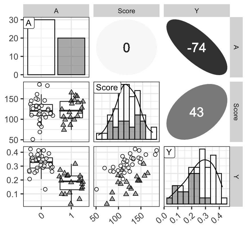
Figure 1: 三個變量的分佈觀察圖,對角線上是三個變量各自的柱狀圖 (histogram) 和計算獲得的概率密度函數曲線;左下角三個圖是三個變量的箱式圖和散點圖;右上角三個圖是三個變量兩兩計算獲得的 Spearman 秩相關乘以100之後的數值。對角線上及左下角三個圖中數據點和形狀的不同分別表示學生喜歡(三角形)和不喜歡(圓形)打工。右上角表示秩相關的數值越接近0,顏色越白圖形越接近圓形,相關係數的絕對值越接近1,則顏色越深,橢圓越細長。
# png(file='output/fig5-1.png', w=1600, h=1600, res=300)
# print(ggp, left=0.3, bottom=0.3)
# dev.off()
Step 2. 寫下數學模型
Model can be written as (Model5-1):
\[ \begin{array}{l} Y[n] = b_1 + b_2A[n] + b_3Sore[n] + \varepsilon [n]& n = 1,2,\dots,N \\ \varepsilon[n] \sim \text{Normal}(0, \sigma) & n = 1,2,\dots,N \\ \end{array} \]
其中,
- \(N\) 表示學生的人數,\(n\)則是學生編號的下標;
- \(b_1\) 是回歸直線的截距;
- \(b_2\) 是\(Score\)保持不變時,\(A\)從\(0\rightarrow 1\)時出勤率的變化(增加,或者減少);
- \(b_3\) 是\(A\)保持不變時,\(Score\)增加一個單位時出勤率的變化(增加,或者減少)。
Model can also be written as (Model5-2):
\[ \begin{array}{l} Y[n] \sim \text{Normal}(b_1 + b_2A[n] + b_3Score[n], \sigma) & n = 1,2,\dots,N \\ \end{array} \]
如果認爲\(A\)和\(Score\)所能預測的出勤率有一個基礎的均值 \(\mu[n]\),剩下的每名學生的出勤率服從這個均值和標準差爲 \(\sigma\) 的正態分佈,那麼模型又可以繼續改寫成爲下面的 Model 5-3:
\[ \begin{array}{l} \mu[n] = b_1 + b_2A[n] + b_3Sore[n] & n = 1,2,\dots,N \\ Y[n] \sim \text{Normal}(\mu[n], \sigma) & n = 1,2,\dots,N \\ \end{array} \]
下面的 Stan 模型是按照 Model 5-3 寫的,它的模型參數有四個,\(b_1, b_2, b_3, \sigma\),\(\mu[n]\)通過 transformed parameter 計算獲得:
data {
  int N;
  int<lower=0, upper=1> A[N];
  real<lower=0, upper=1> Score[N];
  real<lower=0, upper=1> Y[N];
}

parameters {
  real b1;
  real b2;
  real b3;
  real<lower=0> sigma;
}

transformed parameters {
  real mu[N];
  for (n in 1:N) {
    mu[n] = b1 + b2*A[n] + b3*Score[n];
  }
}

model {
  for (n in 1:N) {
    Y[n] ~ normal(mu[n], sigma);
  }
}

generated quantities {
  real y_pred[N];
  for (n in 1:N) {
    y_pred[n] = normal_rng(mu[n], sigma);
  }
}
下面的 R 代碼用來實現對上面 Stan 模型的擬合:
library(rstan)
d <- read.csv(file='https://raw.githubusercontent.com/winterwang/RStanBook/master/chap05/input/data-attendance-1.txt', header = T)
data <- list(N=nrow(d), A=d$A, Score=d$Score/200, Y=d$Y)
fit <- stan(file='stanfiles/model5-3.stan', data=data, seed=1234)
##
## SAMPLING FOR MODEL 'model5-3' NOW (CHAIN 1).
## Chain 1:
## Chain 1: Gradient evaluation took 1.8e-05 seconds
## Chain 1: 1000 transitions using 10 leapfrog steps per transition would take 0.18 seconds.
## Chain 1: Adjust your expectations accordingly!
## Chain 1:
## Chain 1:
## Chain 1: Iteration: 1 / 2000 [ 0%] (Warmup)
## Chain 1: Iteration: 200 / 2000 [ 10%] (Warmup)
## Chain 1: Iteration: 400 / 2000 [ 20%] (Warmup)
## Chain 1: Iteration: 600 / 2000 [ 30%] (Warmup)
## Chain 1: Iteration: 800 / 2000 [ 40%] (Warmup)
## Chain 1: Iteration: 1000 / 2000 [ 50%] (Warmup)
## Chain 1: Iteration: 1001 / 2000 [ 50%] (Sampling)
## Chain 1: Iteration: 1200 / 2000 [ 60%] (Sampling)
## Chain 1: Iteration: 1400 / 2000 [ 70%] (Sampling)
## Chain 1: Iteration: 1600 / 2000 [ 80%] (Sampling)
## Chain 1: Iteration: 1800 / 2000 [ 90%] (Sampling)
## Chain 1: Iteration: 2000 / 2000 [100%] (Sampling)
## Chain 1:
## Chain 1: Elapsed Time: 0.120626 seconds (Warm-up)
## Chain 1: 0.137671 seconds (Sampling)
## Chain 1: 0.258297 seconds (Total)
## Chain 1:
##
## SAMPLING FOR MODEL 'model5-3' NOW (CHAIN 2).
## Chain 2:
## Chain 2: Gradient evaluation took 6e-06 seconds
## Chain 2: 1000 transitions using 10 leapfrog steps per transition would take 0.06 seconds.
## Chain 2: Adjust your expectations accordingly!
## Chain 2:
## Chain 2:
## Chain 2: Iteration: 1 / 2000 [ 0%] (Warmup)
## Chain 2: Iteration: 200 / 2000 [ 10%] (Warmup)
## Chain 2: Iteration: 400 / 2000 [ 20%] (Warmup)
## Chain 2: Iteration: 600 / 2000 [ 30%] (Warmup)
## Chain 2: Iteration: 800 / 2000 [ 40%] (Warmup)
## Chain 2: Iteration: 1000 / 2000 [ 50%] (Warmup)
## Chain 2: Iteration: 1001 / 2000 [ 50%] (Sampling)
## Chain 2: Iteration: 1200 / 2000 [ 60%] (Sampling)
## Chain 2: Iteration: 1400 / 2000 [ 70%] (Sampling)
## Chain 2: Iteration: 1600 / 2000 [ 80%] (Sampling)
## Chain 2: Iteration: 1800 / 2000 [ 90%] (Sampling)
## Chain 2: Iteration: 2000 / 2000 [100%] (Sampling)
## Chain 2:
## Chain 2: Elapsed Time: 0.11864 seconds (Warm-up)
## Chain 2: 0.14427 seconds (Sampling)
## Chain 2: 0.26291 seconds (Total)
## Chain 2:
##
## SAMPLING FOR MODEL 'model5-3' NOW (CHAIN 3).
## Chain 3:
## Chain 3: Gradient evaluation took 7e-06 seconds
## Chain 3: 1000 transitions using 10 leapfrog steps per transition would take 0.07 seconds.
## Chain 3: Adjust your expectations accordingly!
## Chain 3:
## Chain 3:
## Chain 3: Iteration: 1 / 2000 [ 0%] (Warmup)
## Chain 3: Iteration: 200 / 2000 [ 10%] (Warmup)
## Chain 3: Iteration: 400 / 2000 [ 20%] (Warmup)
## Chain 3: Iteration: 600 / 2000 [ 30%] (Warmup)
## Chain 3: Iteration: 800 / 2000 [ 40%] (Warmup)
## Chain 3: Iteration: 1000 / 2000 [ 50%] (Warmup)
## Chain 3: Iteration: 1001 / 2000 [ 50%] (Sampling)
## Chain 3: Iteration: 1200 / 2000 [ 60%] (Sampling)
## Chain 3: Iteration: 1400 / 2000 [ 70%] (Sampling)
## Chain 3: Iteration: 1600 / 2000 [ 80%] (Sampling)
## Chain 3: Iteration: 1800 / 2000 [ 90%] (Sampling)
## Chain 3: Iteration: 2000 / 2000 [100%] (Sampling)
## Chain 3:
## Chain 3: Elapsed Time: 0.125027 seconds (Warm-up)
## Chain 3: 0.122722 seconds (Sampling)
## Chain 3: 0.247749 seconds (Total)
## Chain 3:
##
## SAMPLING FOR MODEL 'model5-3' NOW (CHAIN 4).
## Chain 4:
## Chain 4: Gradient evaluation took 7e-06 seconds
## Chain 4: 1000 transitions using 10 leapfrog steps per transition would take 0.07 seconds.
## Chain 4: Adjust your expectations accordingly!
## Chain 4:
## Chain 4:
## Chain 4: Iteration: 1 / 2000 [ 0%] (Warmup)
## Chain 4: Iteration: 200 / 2000 [ 10%] (Warmup)
## Chain 4: Iteration: 400 / 2000 [ 20%] (Warmup)
## Chain 4: Iteration: 600 / 2000 [ 30%] (Warmup)
## Chain 4: Iteration: 800 / 2000 [ 40%] (Warmup)
## Chain 4: Iteration: 1000 / 2000 [ 50%] (Warmup)
## Chain 4: Iteration: 1001 / 2000 [ 50%] (Sampling)
## Chain 4: Iteration: 1200 / 2000 [ 60%] (Sampling)
## Chain 4: Iteration: 1400 / 2000 [ 70%] (Sampling)
## Chain 4: Iteration: 1600 / 2000 [ 80%] (Sampling)
## Chain 4: Iteration: 1800 / 2000 [ 90%] (Sampling)
## Chain 4: Iteration: 2000 / 2000 [100%] (Sampling)
## Chain 4:
## Chain 4: Elapsed Time: 0.129317 seconds (Warm-up)
## Chain 4: 0.13154 seconds (Sampling)
## Chain 4: 0.260857 seconds (Total)
## Chain 4:fit## Inference for Stan model: model5-3.
## 4 chains, each with iter=2000; warmup=1000; thin=1;
## post-warmup draws per chain=1000, total post-warmup draws=4000.
##
## mean se_mean sd 2.5% 25% 50% 75% 97.5% n_eff Rhat
## b1 0.12 0.00 0.03 0.06 0.10 0.12 0.15 0.19 1803 1
## b2 -0.14 0.00 0.01 -0.17 -0.15 -0.14 -0.13 -0.11 2486 1
## b3 0.32 0.00 0.05 0.22 0.29 0.33 0.36 0.43 1751 1
## sigma 0.05 0.00 0.01 0.04 0.05 0.05 0.05 0.06 2328 1
## mu[1] 0.24 0.00 0.02 0.20 0.22 0.24 0.25 0.27 2014 1
## mu[2] 0.22 0.00 0.01 0.19 0.21 0.22 0.22 0.24 2589 1
## mu[3] 0.33 0.00 0.01 0.31 0.32 0.33 0.33 0.35 3512 1
## mu[4] 0.12 0.00 0.02 0.09 0.11 0.12 0.13 0.15 2338 1
## mu[5] 0.24 0.00 0.02 0.21 0.23 0.24 0.25 0.27 2333 1
## mu[6] 0.34 0.00 0.01 0.32 0.33 0.34 0.35 0.36 3369 1
## mu[7] 0.30 0.00 0.01 0.28 0.30 0.30 0.31 0.32 3110 1
## mu[8] 0.22 0.00 0.01 0.19 0.21 0.22 0.23 0.24 2544 1
## mu[9] 0.36 0.00 0.01 0.34 0.35 0.36 0.37 0.38 2891 1
## mu[10] 0.36 0.00 0.01 0.34 0.35 0.36 0.37 0.38 2926 1
## mu[11] 0.21 0.00 0.01 0.18 0.20 0.21 0.22 0.23 2683 1
## mu[12] 0.35 0.00 0.01 0.33 0.34 0.35 0.35 0.37 3228 1
## mu[13] 0.17 0.00 0.01 0.15 0.16 0.17 0.18 0.19 2964 1
## mu[14] 0.30 0.00 0.01 0.28 0.30 0.30 0.31 0.32 3110 1
## mu[15] 0.30 0.00 0.01 0.28 0.29 0.30 0.31 0.32 3017 1
## mu[16] 0.14 0.00 0.01 0.12 0.13 0.14 0.15 0.17 2577 1
## mu[17] 0.31 0.00 0.01 0.29 0.30 0.31 0.31 0.33 3244 1
## mu[18] 0.26 0.00 0.01 0.23 0.25 0.26 0.27 0.28 2168 1
## mu[19] 0.42 0.00 0.02 0.38 0.41 0.42 0.44 0.46 2180 1
## mu[20] 0.23 0.00 0.01 0.20 0.22 0.23 0.24 0.26 2367 1
## mu[21] 0.12 0.00 0.02 0.09 0.11 0.12 0.13 0.15 2338 1
## mu[22] 0.16 0.00 0.01 0.13 0.15 0.16 0.16 0.18 2789 1
## mu[23] 0.15 0.00 0.01 0.13 0.14 0.15 0.16 0.18 2743 1
## mu[24] 0.21 0.00 0.01 0.19 0.20 0.21 0.22 0.24 2635 1
## mu[25] 0.17 0.00 0.01 0.15 0.16 0.17 0.18 0.19 2953 1
## mu[26] 0.19 0.00 0.01 0.16 0.18 0.19 0.20 0.21 2961 1
## mu[27] 0.32 0.00 0.01 0.30 0.31 0.32 0.32 0.34 3426 1
## mu[28] 0.32 0.00 0.01 0.30 0.31 0.32 0.32 0.34 3426 1
## mu[29] 0.38 0.00 0.01 0.36 0.38 0.39 0.39 0.41 2484 1
## mu[30] 0.31 0.00 0.01 0.29 0.30 0.31 0.31 0.33 3200 1
## mu[31] 0.25 0.00 0.02 0.22 0.24 0.25 0.26 0.28 2232 1
## mu[32] 0.10 0.00 0.02 0.07 0.09 0.10 0.11 0.14 2185 1
## mu[33] 0.20 0.00 0.01 0.18 0.20 0.20 0.21 0.23 2754 1
## mu[34] 0.18 0.00 0.01 0.16 0.17 0.18 0.19 0.20 2989 1
## mu[35] 0.33 0.00 0.01 0.31 0.32 0.33 0.33 0.35 3509 1
## mu[36] 0.34 0.00 0.01 0.32 0.33 0.34 0.34 0.36 3427 1
## mu[37] 0.15 0.00 0.01 0.13 0.14 0.15 0.16 0.18 2719 1
## mu[38] 0.30 0.00 0.01 0.28 0.30 0.30 0.31 0.32 3064 1
## mu[39] 0.27 0.00 0.01 0.24 0.26 0.27 0.28 0.29 2306 1
## mu[40] 0.27 0.00 0.01 0.24 0.26 0.27 0.27 0.29 2283 1
## mu[41] 0.33 0.00 0.01 0.31 0.33 0.33 0.34 0.35 3472 1
## mu[42] 0.34 0.00 0.01 0.32 0.33 0.34 0.35 0.36 3369 1
## mu[43] 0.32 0.00 0.01 0.30 0.32 0.32 0.33 0.34 3491 1
## mu[44] 0.36 0.00 0.01 0.34 0.36 0.36 0.37 0.39 2823 1
## mu[45] 0.42 0.00 0.02 0.38 0.41 0.42 0.43 0.45 2204 1
## mu[46] 0.29 0.00 0.01 0.27 0.29 0.29 0.30 0.31 2838 1
## mu[47] 0.21 0.00 0.02 0.17 0.19 0.21 0.22 0.25 1910 1
## mu[48] 0.37 0.00 0.01 0.34 0.36 0.37 0.38 0.39 2759 1
## mu[49] 0.28 0.00 0.01 0.26 0.28 0.28 0.29 0.31 2603 1
## mu[50] 0.14 0.00 0.01 0.12 0.13 0.14 0.15 0.17 2577 1
## y_pred[1] 0.23 0.00 0.05 0.13 0.20 0.23 0.27 0.34 3730 1
## y_pred[2] 0.22 0.00 0.05 0.11 0.18 0.22 0.25 0.32 3977 1
## y_pred[3] 0.32 0.00 0.05 0.23 0.29 0.32 0.36 0.43 3856 1
## y_pred[4] 0.12 0.00 0.05 0.01 0.08 0.12 0.15 0.22 3896 1
## y_pred[5] 0.24 0.00 0.05 0.13 0.20 0.24 0.27 0.34 3804 1
## y_pred[6] 0.34 0.00 0.05 0.24 0.31 0.34 0.38 0.44 3865 1
## y_pred[7] 0.30 0.00 0.05 0.20 0.27 0.30 0.34 0.41 3757 1
## y_pred[8] 0.22 0.00 0.05 0.11 0.18 0.22 0.25 0.33 3784 1
## y_pred[9] 0.36 0.00 0.05 0.26 0.33 0.36 0.40 0.47 3939 1
## y_pred[10] 0.36 0.00 0.05 0.25 0.32 0.36 0.39 0.46 3743 1
## y_pred[11] 0.21 0.00 0.05 0.10 0.17 0.21 0.25 0.32 4113 1
## y_pred[12] 0.35 0.00 0.05 0.24 0.31 0.35 0.38 0.45 4149 1
## y_pred[13] 0.17 0.00 0.05 0.07 0.14 0.17 0.21 0.28 3806 1
## y_pred[14] 0.30 0.00 0.05 0.20 0.27 0.30 0.34 0.41 3944 1
## y_pred[15] 0.30 0.00 0.05 0.20 0.27 0.30 0.34 0.41 3930 1
## y_pred[16] 0.14 0.00 0.05 0.03 0.11 0.14 0.18 0.24 3833 1
## y_pred[17] 0.31 0.00 0.05 0.21 0.27 0.31 0.34 0.41 3981 1
## y_pred[18] 0.26 0.00 0.05 0.15 0.22 0.26 0.29 0.37 3718 1
## y_pred[19] 0.43 0.00 0.06 0.32 0.39 0.43 0.46 0.53 3690 1
## y_pred[20] 0.23 0.00 0.05 0.13 0.20 0.23 0.27 0.34 2926 1
## y_pred[21] 0.12 0.00 0.05 0.01 0.08 0.12 0.15 0.23 3751 1
## y_pred[22] 0.16 0.00 0.05 0.05 0.12 0.16 0.19 0.26 3993 1
## y_pred[23] 0.15 0.00 0.05 0.04 0.11 0.15 0.19 0.26 3990 1
## y_pred[24] 0.21 0.00 0.05 0.11 0.17 0.21 0.25 0.32 3766 1
## y_pred[25] 0.17 0.00 0.05 0.06 0.13 0.17 0.21 0.27 3800 1
## y_pred[26] 0.19 0.00 0.05 0.08 0.15 0.19 0.22 0.30 3781 1
## y_pred[27] 0.32 0.00 0.05 0.22 0.28 0.32 0.35 0.42 4073 1
## y_pred[28] 0.32 0.00 0.05 0.21 0.28 0.32 0.35 0.42 4155 1
## y_pred[29] 0.38 0.00 0.05 0.28 0.35 0.38 0.42 0.49 3869 1
## y_pred[30] 0.31 0.00 0.05 0.20 0.27 0.31 0.34 0.41 3708 1
## y_pred[31] 0.25 0.00 0.06 0.14 0.21 0.25 0.29 0.35 4005 1
## y_pred[32] 0.10 0.00 0.06 -0.01 0.06 0.10 0.14 0.21 3479 1
## y_pred[33] 0.20 0.00 0.05 0.10 0.17 0.20 0.24 0.31 3656 1
## y_pred[34] 0.18 0.00 0.05 0.08 0.15 0.18 0.22 0.28 4111 1
## y_pred[35] 0.33 0.00 0.05 0.22 0.29 0.33 0.36 0.43 3866 1
## y_pred[36] 0.34 0.00 0.05 0.23 0.30 0.34 0.37 0.44 4043 1
## y_pred[37] 0.15 0.00 0.05 0.04 0.12 0.15 0.19 0.25 3830 1
## y_pred[38] 0.30 0.00 0.05 0.20 0.27 0.30 0.34 0.41 3814 1
## y_pred[39] 0.27 0.00 0.05 0.16 0.23 0.27 0.30 0.37 3792 1
## y_pred[40] 0.27 0.00 0.05 0.16 0.23 0.27 0.30 0.37 3793 1
## y_pred[41] 0.33 0.00 0.05 0.23 0.30 0.33 0.37 0.44 3748 1
## y_pred[42] 0.34 0.00 0.05 0.23 0.30 0.34 0.38 0.44 3811 1
## y_pred[43] 0.32 0.00 0.05 0.22 0.29 0.32 0.35 0.42 4268 1
## y_pred[44] 0.36 0.00 0.05 0.26 0.33 0.36 0.40 0.47 4015 1
## y_pred[45] 0.42 0.00 0.05 0.31 0.38 0.42 0.45 0.53 3658 1
## y_pred[46] 0.29 0.00 0.05 0.19 0.26 0.29 0.33 0.40 3993 1
## y_pred[47] 0.21 0.00 0.06 0.10 0.17 0.21 0.24 0.32 3671 1
## y_pred[48] 0.37 0.00 0.05 0.26 0.33 0.37 0.40 0.47 3988 1
## y_pred[49] 0.28 0.00 0.05 0.18 0.25 0.28 0.32 0.39 3596 1
## y_pred[50] 0.14 0.00 0.05 0.03 0.10 0.14 0.18 0.24 4027 1
## lp__ 120.85 0.04 1.43 117.36 120.12 121.19 121.90 122.68 1610 1
##
## Samples were drawn using NUTS(diag_e) at Mon May 18 16:52:55 2020.
## For each parameter, n_eff is a crude measure of effective sample size,
## and Rhat is the potential scale reduction factor on split chains (at
## convergence, Rhat=1).上述代碼中值得注意的是我們對 \(Score\) 進行了全部除以 \(200\) 的數據縮放調整 (scaling)。這樣有助於我們的模型在進行 MCMC 計算時加速其達到收斂時所需要的時間。
把計算獲得的事後模型參數平均值代入模型 Model 5-3:
\[ \begin{array}{l} \mu[n] = 0.12 - 0.14A[n] + 0.32Sore[n] & n = 1,2,\dots,N \\ Y[n] \sim \text{Normal}(\mu[n], 0.05) & n = 1,2,\dots,N \\ \end{array} \]
從輸出的結果報告來看,所有的 Rhat 都小於1.1,可以認爲採樣已經達到收斂效果,再來確認一下軌跡圖:
library(bayesplot)

color_scheme_set("mix-brightblue-gray")

posterior2 <- rstan::extract(fit, inc_warmup = TRUE, permuted = FALSE)

p <- mcmc_trace(posterior2, n_warmup = 0, pars = c("b1", "b2", "b3", "sigma", "lp__"),
                facet_args = list(nrow = 2, labeller = label_parsed))
p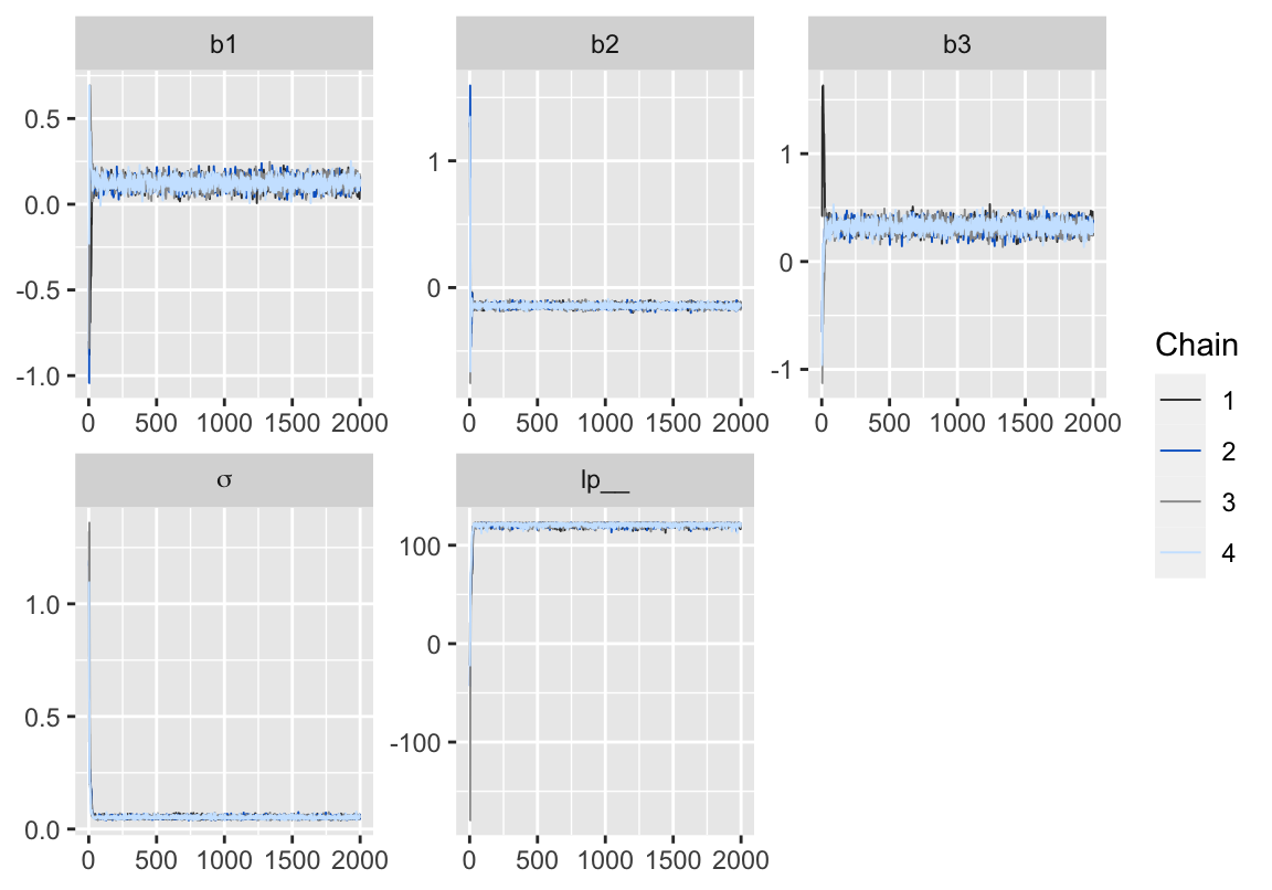
Figure 2: 用 bayesplot包數繪製的模型5-3的MCMC鏈式軌跡圖 (trace plot)。
收斂效果很不錯,下面來解釋回歸係數的事後均值的涵義:
b3的事後均值是\(0.32\),所以,\(Score=150\)和\(Score=50\)的兩名學生,當他們同時都是喜歡或者同時都不喜歡打工時,\(Score = 150\)的學生的出勤率平均比 \(Score = 50\) 的學生的出勤率高 \(0.32 \times (150-50)/200 = 0.16\)。b2的事後均值是\(-0.14\),所以,同樣地,\(Score\)相同的兩名學生,喜歡打工的學生比不喜歡打工的學生出勤率平均要低 \(0.14\)。
Step 3. 看圖確認模型擬合狀況
下圖繪製了上面貝葉斯多重線性回歸模型計算獲得的事後貝葉斯預測區間,和觀測值\(Y\)出勤率之間的直觀關係:
source("commonRstan.R")

ms <- rstan::extract(fit)

Score_new <- 50:200
N_X <- length(Score_new)
N_mcmc <- length(ms$lp__)

set.seed(1234)
y_base_mcmc <- as.data.frame(matrix(nrow=N_mcmc, ncol=N_X))
y_base_a0_mcmc <- as.data.frame(matrix(nrow = N_mcmc, ncol = N_X))
y_mcmc <- as.data.frame(matrix(nrow=N_mcmc, ncol=N_X))
y_a0_mcmc <- as.data.frame(matrix(nrow=N_mcmc, ncol=N_X))

for (i in 1:N_X) {
  y_base_mcmc[,i] <- ms$b1 + ms$b2 + ms$b3 * Score_new[i]/200
  y_base_a0_mcmc[] <- ms$b1 + ms$b2*0 + ms$b3 * Score_new[i]/200
  y_mcmc[,i] <- rnorm(n=N_mcmc, mean=y_base_mcmc[,i], sd=ms$sigma)
  y_a0_mcmc[,i] <- rnorm(n=N_mcmc, mean=y_base_a0_mcmc[,i], sd=ms$sigma)
}

customize.ggplot.axis <- function(p) {
  p <- p + labs(x='Score', y='Y')
  p <- p + scale_y_continuous(breaks=seq(from=-0.2, to=0.8, by=0.2))
  p <- p + coord_cartesian(xlim=c(50, 200), ylim=c(-0.2, 0.6))
  return(p)
}

d_est <- data.frame.quantile.mcmc(x=Score_new, y_mcmc=y_mcmc)
d_esta0 <- data.frame.quantile.mcmc(x=Score_new, y_mcmc=y_a0_mcmc)
# p <- ggplot.5quantile(data=d_est)
# p2 <- ggplot.5quantile(data = d_esta0)
# p <- p + geom_point(data=d[d$A==1, ], aes(x=Score, y=Y), shape=24, size=5)
# p2 <- p2 + geom_point(data=d[d$A==0, ], aes(x=Score, y=Y), shape=1, size=5)
# p <- customize.ggplot.axis(p)
# p2 <- customize.ggplot.axis(p2)

visuals = rbind(d_est,d_esta0)
visuals$A=c(rep(1,151),rep(0,151)) # 151 points of each flavour

qn <- colnames(visuals)[-1]
p <- ggplot(data=visuals, aes(x=X, y=p50, group = A))
p <- p + my_theme()
p <- p + geom_ribbon(aes_string(ymin=qn[1], ymax=qn[5]), fill='black', alpha=1/6)
p <- p + geom_ribbon(aes_string(ymin=qn[2], ymax=qn[4]), fill='black', alpha=2/6)
p <- p + geom_line(size=1)
p <- p + geom_point(data=d[d$A==1, ], aes(x=Score, y=Y), shape=24, size=5)
p <- p + geom_point(data=d[d$A==0, ], aes(x=Score, y=Y), shape=20, size=5)
p <- customize.ggplot.axis(p)
p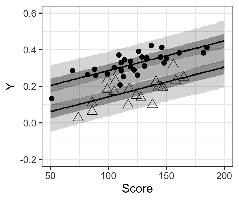
Figure 3: 黑色原點(不喜歡打工),和無色三角形(喜歡打工)的學生的出勤率,和模型計算獲得的貝葉斯事後預測區間。黑色線是中位數,灰色帶是50%預測區間和95%預測區間。
上述觀察預測值區間和實際觀測之間的關係的視覺化圖形,在多重線性回歸模型只有兩個預測變量的事後還較爲容易獲得,當模型中有三個或以上的預測變量時,可視化變得困難重重。
此時我們推薦繪製“實際觀測值和預測值”,以及模型給出的每個預測值的隨機誤差\(\varepsilon\)分佈範圍,相結合的圖形來判斷模型擬合程度。
d_qua <- t(apply(ms$y_pred, 2, quantile, prob=c(0.1, 0.5, 0.9)))
colnames(d_qua) <- c('p10', 'p50', 'p90')
d_qua <- data.frame(d, d_qua)
d_qua$A <- as.factor(d_qua$A)

p <- ggplot(data=d_qua, aes(x=Y, y=p50, ymin=p10, ymax=p90, shape=A, fill=A))
p <- p + theme_bw(base_size=18) + theme(legend.key.height=grid::unit(2.5,'line'))
p <- p + coord_fixed(ratio=1, xlim=c(0, 0.5), ylim=c(0, 0.5))
p <- p + geom_pointrange(size=0.8, color='grey5')
p <- p + geom_abline(aes(slope=1, intercept=0), color='black', alpha=3/5, linetype='31')
p <- p + scale_shape_manual(values=c(21, 24))
p <- p + scale_fill_manual(values=c('white', 'grey70'))
p <- p + labs(x='Observed', y='Predicted')
p <- p + scale_x_continuous(breaks=seq(from=0, to=0.5, by=0.1))
p <- p + scale_y_continuous(breaks=seq(from=0, to=0.5, by=0.1))
p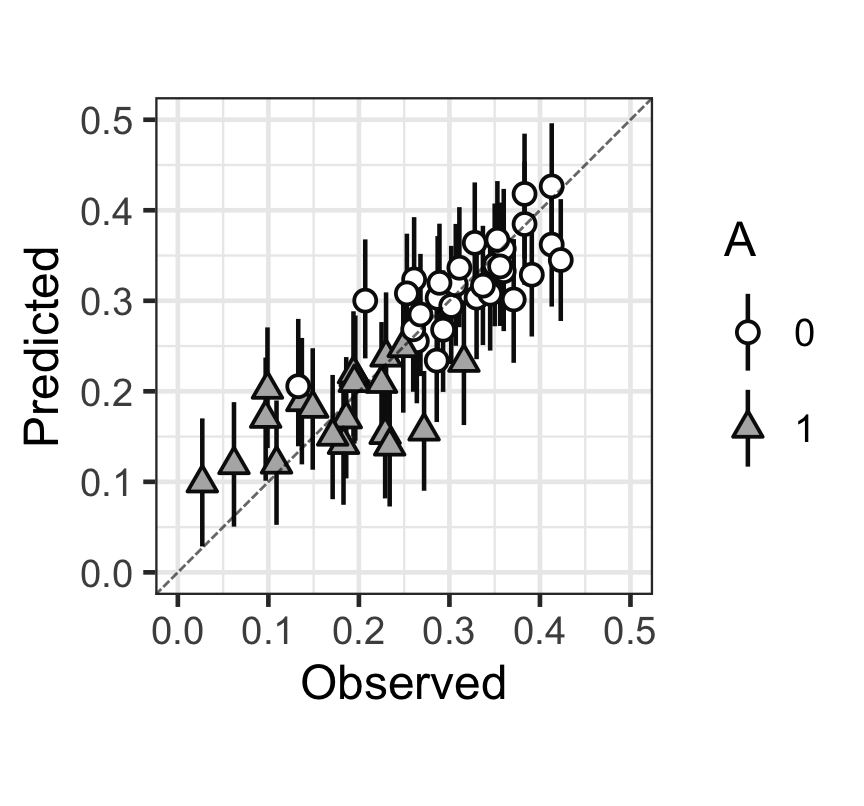
Figure 4: 觀測值(x),和預測值(y)的散點圖,以及預測值的80%預測區間。
從上圖中可以看出,大多數的觀測點和預測點以及預測的80%區間基本都在 \(y = x\) 這條對角線上。大致可以認爲本次貝葉斯多重線性回歸擬合效果尚且能夠接受。
隨機誤差 \(\varepsilon[n]\) 被認爲服從 \(\text{Normal}(0, \sigma)\) 的正態分佈。從模型中可以計算獲得每個學生出勤率的預測值和實際觀測值之間的差,這就是隨機誤差。貝葉斯框架之下,我們實際獲得的會是每名學生隨機誤差的分佈:
N_mcmc <- length(ms$lp__)

d_noise <- data.frame(t(-t(ms$mu) + d$Y))
colnames(d_noise) <- paste0('noise', 1:nrow(d))
d_est <- data.frame(mcmc=1:N_mcmc, d_noise)
d_melt <- reshape2::melt(d_est, id=c('mcmc'), variable.name='X')

d_mode <- data.frame(t(apply(d_noise, 2, function(x) {
  dens <- density(x)
  mode_i <- which.max(dens$y)
  mode_x <- dens$x[mode_i]
  mode_y <- dens$y[mode_i]
  c(mode_x, mode_y)
})))
colnames(d_mode) <- c('X', 'Y')

p <- ggplot()
p <- p + theme_bw(base_size=18)
p <- p + geom_line(data=d_melt, aes(x=value, group=X), stat='density', color='black', alpha=0.4)
p <- p + geom_segment(data=d_mode, aes(x=X, xend=X, y=Y, yend=0), color='black', linetype='dashed', alpha=0.4)
p <- p + geom_rug(data=d_mode, aes(x=X), sides='b')
p <- p + labs(x='value', y='density')
p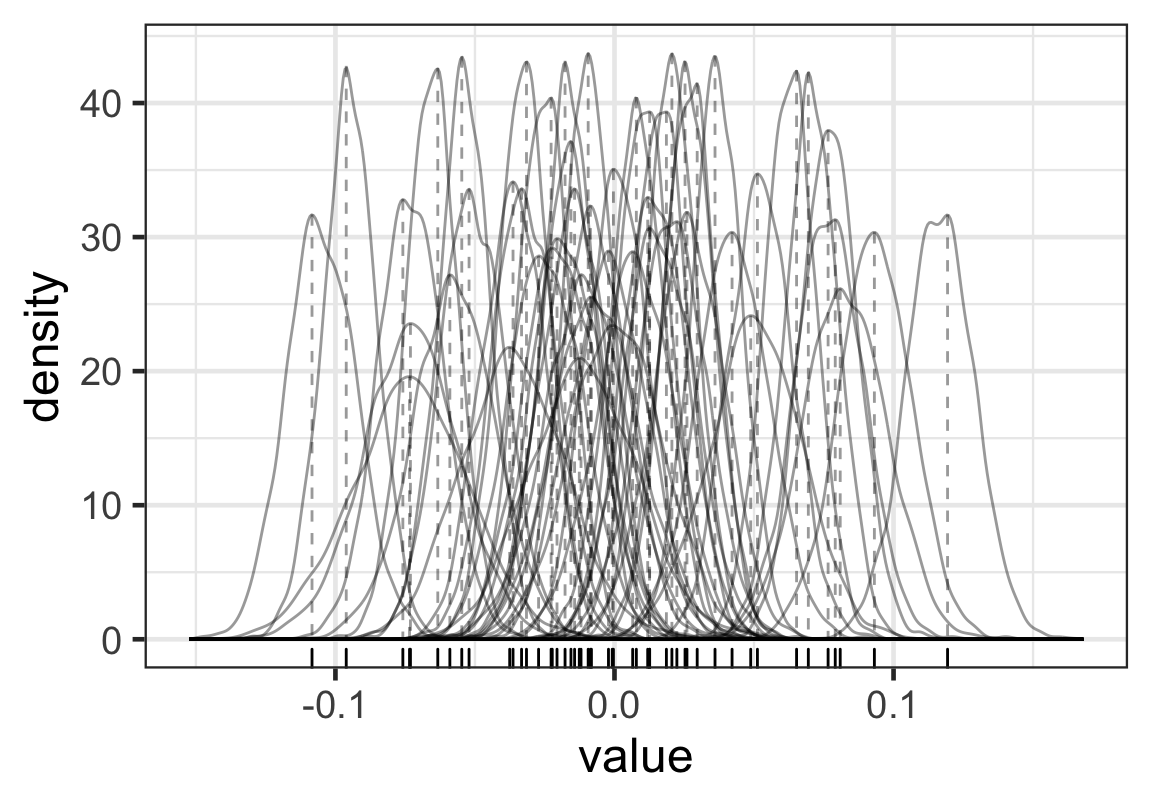
Figure 5: 每名學生的出勤率隨機誤差的分佈
實際上我們只需要選取每名學生模型計算獲得的事後隨機誤差的代表值,比如可以是平均值,中央值,或者是MAP值(事後確率最大推定値,maximum a posteriori estimate),來觀察就可以了:
s_dens <- density(ms$s)
s_MAP <- s_dens$x[which.max(s_dens$y)]
bw <- 0.01
p <- ggplot(data=d_mode, aes(x=X))
p <- p + theme_bw(base_size=18)
p <- p + geom_histogram(binwidth=bw, color='black', fill='white')
p <- p + geom_density(eval(bquote(aes(y=..count..*.(bw)))), alpha=0.5, color='black', fill='gray20')
p <- p + stat_function(fun=function(x) nrow(d)*bw*dnorm(x, mean=0, sd=s_MAP), linetype='dashed')
p <- p + labs(x='value', y='count')
p <- p + xlim(range(density(d_mode$X)$x))
p
## Warning: Removed 2 rows containing missing values (geom_bar).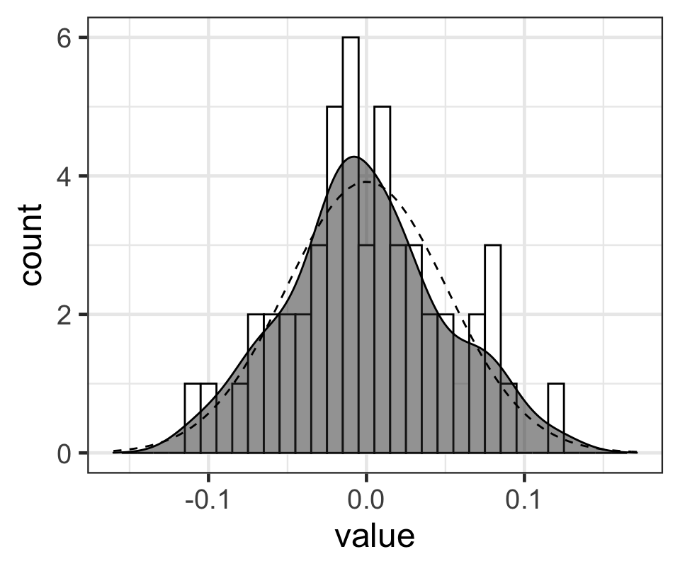
Figure 6: 每名學生事後出勤率隨機誤差的MAP值的柱狀圖,和相應的概率密度函數(灰色鐘罩),點狀虛線是均值爲0,標準差是模型計算的事後隨機誤差標準差的 MAP 值的正態分佈的形狀。
Step 4. MCMC 樣本的散點圖矩陣
library(ggplot2)
library(GGally)
library(hexbin)


d <- data.frame(b1=ms$b1, b2=ms$b2, b3=ms$b3, sigma=ms$sigma, mu1=ms$mu[,1], mu50=ms$mu[,50], lp__=ms$lp__)
N_col <- ncol(d)
ggp <- ggpairs(d, upper='blank', diag='blank', lower='blank')

label_list <- list(b1='b1', b2='b2', b3='b3', sigma='sigma', mu1='mu[1]', mu50='mu[50]', lp__='lp__')
for(i in 1:N_col) {
  x <- d[,i]
  bw <- (max(x)-min(x))/10
  p <- ggplot(data.frame(x), aes(x))
  p <- p + theme_bw(base_size=14)
  p <- p + theme(axis.text.x=element_text(angle=60, vjust=1, hjust=1))
  p <- p + geom_histogram(binwidth=bw, fill='white', color='grey5')
  p <- p + geom_line(eval(bquote(aes(y=..count..*.(bw)))), stat='density')
  p <- p + geom_label(data=data.frame(x=-Inf, y=Inf, label=label_list[[colnames(d)[i]]]), aes(x=x, y=y, label=label), hjust=0, vjust=1)
  ggp <- putPlot(ggp, p, i, i)
}

zcolat <- seq(-1, 1, length=81)
zcolre <- c(zcolat[1:40]+1, rev(zcolat[41:81]))

for(i in 1:(N_col-1)) {
  for(j in (i+1):N_col) {
    x <- as.numeric(d[,i])
    y <- as.numeric(d[,j])
    r <- cor(x, y, method='spearman', use='pairwise.complete.obs')
    zcol <- lattice::level.colors(r, at=zcolat, col.regions=grey(zcolre))
    textcol <- ifelse(abs(r) < 0.4, 'grey20', 'white')
    ell <- ellipse::ellipse(r, level=0.95, type='l', npoints=50, scale=c(.2, .2), centre=c(.5, .5))
    p <- ggplot(data.frame(ell), aes(x=x, y=y))
    p <- p + theme_bw() + theme(
      plot.background=element_blank(),
      panel.grid.major=element_blank(), panel.grid.minor=element_blank(),
      panel.border=element_blank(), axis.ticks=element_blank()
    )
    p <- p + geom_polygon(fill=zcol, color=zcol)
    p <- p + geom_text(data=NULL, x=.5, y=.5, label=100*round(r, 2), size=6, col=textcol)
    ggp <- putPlot(ggp, p, i, j)
  }
}

for(j in 1:(N_col-1)) {
  for(i in (j+1):N_col) {
    x <- d[,j]
    y <- d[,i]
    p <- ggplot(data.frame(x, y), aes(x=x, y=y))
    p <- p + theme_bw(base_size=14)
    p <- p + theme(axis.text.x=element_text(angle=60, vjust=1, hjust=1))
    p <- p + geom_hex()
    p <- p + scale_fill_gradientn(colours=gray.colors(7, start=0.1, end=0.9))
    ggp <- putPlot(ggp, p, i, j)
  }
}
ggp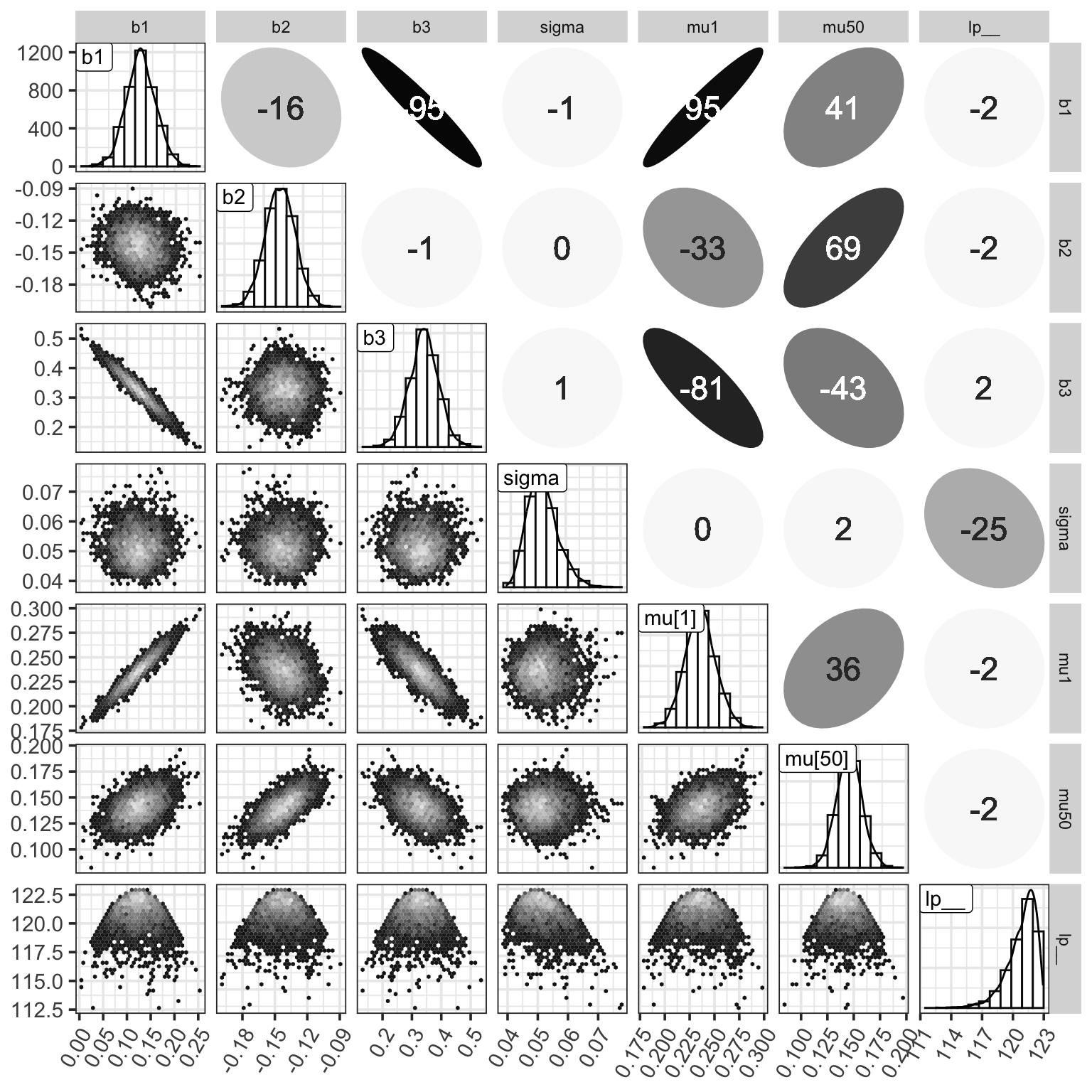
Figure 7: MCMC樣本的事後矩陣。對角線上是各個參數事後樣本的柱狀圖和相應的概率密度曲線。右上角是各個參數事後樣本之間的 Spearman 秩相關係數。左下角是兩兩的散點圖。